Где находится порядковый номер

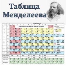
Графическим отображением периодического закона является Периодическая система химических элементов. Известно более (700) форм периодической таблицы. Официальным по решению Международного союза химиков является её полудлинный вариант.

Рис. (1). Периодическая система химических элементов

Каждому химическому элементу в таблице отведена одна клеточка, в которой указаны символ и название элемента, порядковый номер и относительная атомная масса.

Ломаная линия обозначает границу между металлами и неметаллами.

Последовательность расположения элементов не всегда совпадает с возрастанием атомной массы. Есть несколько исключений из правила. Так, относительная атомная масса аргона больше атомной массы калия, в теллура — больше, чем йода.

Каждый элемент имеет свой порядковый (атомный) номер, располагается в определённом периоде и определённой группе.

В таблице семь периодов. В каждом содержится определённое число элементов:

(1)-й период — (2) элемента,

(2)-й период — (8) элементов,

(3)-й период — (8) элементов,

(4)-й период — (18) элементов,

(5)-й период — (18) элементов,

(6)-й период — (32) элемента ((18 + 14)),

(7)-й период — (32) элемента ((18 + 14)).

Три первых периода называют малыми периодами, остальные — большими. И в малых, и в больших периодах происходит постепенное ослабление металлических свойств и усиление неметаллических, только в больших периодах оно происходит более плавно.

Восьмой период появится в Периодической таблице, когда будут открыты новые элементы.

В Периодической таблице (18) групп, пронумерованных арабскими цифрами. Часто используют нумерацию римскими цифрами с добавлением букв (A) или (B). В таком случае групп (8).

Группы (A) начинаются элементами малых периодов, включают также и элементы больших периодов; содержат и металлы, и неметаллы. В коротком варианте Периодической таблицы это главные подгруппы.

Группы (B) содержат элементы больших периодов, и это только металлы. В коротком варианте Периодической таблицы это побочные подгруппы.

Число элементов в группах:

VIIIB — (12) элементов;

Количественный состав групп будет изменяться по мере добавления в таблицу новых элементов.

Римский номер группы, как правило, показывает высшую валентность в оксидах. Но для некоторых элементов это правило не выполняется. Так, фтор не бывает семивалентным, а кислород — шестивалентным. Не проявляют валентность, равную номеру группы, гелий, неон и аргон — эти элементы не образуют соединений с кислородом. Медь бывает двухвалентной, а золото — трёхвалентным, хотя это элементы первой группы.

Некоторые группы (A) получили особые названия:

This article is about the mathematical concept. For number words denoting a position in a sequence («first», «second», «third», etc.), see Ordinal numeral.

In set theory, an ordinal number, or ordinal, is a generalization of ordinal numerals (first, second, nth, etc.) aimed to extend enumeration to infinite sets.^[1]

A finite set can be enumerated by successively labeling each element with the least natural number that has not been previously used. To extend this process to various infinite sets, ordinal numbers are defined more generally as linearly ordered labels that include the natural numbers and have the property that every set of ordinals has a least element (this is needed for giving a meaning to «the least unused element»).^[2] This more general definition allows us to define an ordinal number (omega) that is greater than every natural number, along with ordinal numbers , , etc., which are even greater than .

A linear order such that every subset has a least element is called a well-order. The axiom of choice implies that every set can be well-ordered, and given two well-ordered sets, one is isomorphic to an initial segment of the other. So ordinal numbers exist and are essentially unique.

Ordinal numbers are distinct from cardinal numbers, which measure the size of sets. Although the distinction between ordinals and cardinals is not always apparent on finite sets (one can go from one to the other just by counting labels), they are very different in the infinite case, where different infinite ordinals can correspond to sets having the same cardinal. Like other kinds of numbers, ordinals can be added, multiplied, and exponentiated, although none of these operations are commutative.

Ordinals were introduced by Georg Cantor in 1883^[3] in order to accommodate infinite sequences and classify derived sets, which he had previously introduced in 1872 while studying the uniqueness of trigonometric series.^[4]

Ordinals extend the natural numbers[edit]

A natural number (which, in this context, includes the number 0) can be used for two purposes: to describe the size of a set, or to describe the position of an element in a sequence. When restricted to finite sets, these two concepts coincide, since all linear orders of a finite set are isomorphic.

When dealing with infinite sets, however, one has to distinguish between the notion of size, which leads to cardinal numbers, and the notion of position, which leads to the ordinal numbers described here. This is because while any set has only one size (its cardinality), there are many nonisomorphic well-orderings of any infinite set, as explained below.

Whereas the notion of cardinal number is associated with a set with no particular structure on it, the ordinals are intimately linked with the special kind of sets that are called well-ordered. A well-ordered set is a totally ordered set in which every non-empty subset has a least element (a totally ordered set is an ordered set such that, given two distinct elements, one is less than the other). Equivalently, assuming the axiom of dependent choice, it is a totally ordered set without any infinite decreasing sequence — though there may be infinite increasing sequences. Ordinals may be used to label the elements of any given well-ordered set (the smallest element being labelled 0, the one after that 1, the next one 2, «and so on»), and to measure the «length» of the whole set by the least ordinal that is not a label for an element of the set. This «length» is called the order type of the set.

Any ordinal is defined by the set of ordinals that precede it. In fact, the most common definition of ordinals identifies each ordinal as the set of ordinals that precede it. For example, the ordinal 42 is generally identified as the set {0, 1, 2, …, 41}. Conversely, any set S of ordinals that is downward closed — meaning that for any ordinal α in S and any ordinal β < α, β is also in S — is (or can be identified with) an ordinal.

This definition of ordinals in terms of sets allows for infinite ordinals. The smallest infinite ordinal is , which can be identified with the set of natural numbers (so that the ordinal associated with every natural number precedes ). Indeed, the set of natural numbers is well-ordered—as is any set of ordinals—and since it is downward closed, it can be identified with the ordinal associated with it.

Perhaps a clearer intuition of ordinals can be formed by examining a first few of them: as mentioned above, they start with the natural numbers, 0, 1, 2, 3, 4, 5, … After all natural numbers comes the first infinite ordinal, ω, and after that come ω+1, ω+2, ω+3, and so on. (Exactly what addition means will be defined later on: just consider them as names.) After all of these come ω·2 (which is ω+ω), ω·2+1, ω·2+2, and so on, then ω·3, and then later on ω·4. Now the set of ordinals formed in this way (the ω·m+n, where m and n are natural numbers) must itself have an ordinal associated with it: and that is ω². Further on, there will be ω³, then ω⁴, and so on, and ω^ω, then ω^ωω, then later ω^ωωω, and even later ε₀ (epsilon nought) (to give a few examples of relatively small—countable—ordinals). This can be continued indefinitely (as every time one says «and so on» when enumerating ordinals, it defines a larger ordinal). The smallest uncountable ordinal is the set of all countable ordinals, expressed as ω₁ or .^[5][6]

Definitions[edit]

Well-ordered sets[edit]

In a well-ordered set, every non-empty subset contains a distinct smallest element. Given the axiom of dependent choice, this is equivalent to saying that the set is totally ordered and there is no infinite decreasing sequence (the latter being easier to visualize). In practice, the importance of well-ordering is justified by the possibility of applying transfinite induction, which says, essentially, that any property that passes on from the predecessors of an element to that element itself must be true of all elements (of the given well-ordered set). If the states of a computation (computer program or game) can be well-ordered—in such a way that each step is followed by a «lower» step—then the computation will terminate.

It is inappropriate to distinguish between two well-ordered sets if they only differ in the «labeling of their elements», or more formally: if the elements of the first set can be paired off with the elements of the second set such that if one element is smaller than another in the first set, then the partner of the first element is smaller than the partner of the second element in the second set, and vice versa. Such a one-to-one correspondence is called an order isomorphism, and the two well-ordered sets are said to be order-isomorphic or similar (with the understanding that this is an equivalence relation).

Formally, if a partial order ≤ is defined on the set S, and a partial order ≤’ is defined on the set S’ , then the posets (S,≤) and (S’ ,≤’) are order isomorphic if there is a bijection f that preserves the ordering. That is, f(a) ≤’ f(b) if and only if a ≤ b. Provided there exists an order isomorphism between two well-ordered sets, the order isomorphism is unique: this makes it quite justifiable to consider the two sets as essentially identical, and to seek a «canonical» representative of the isomorphism type (class). This is exactly what the ordinals provide, and it also provides a canonical labeling of the elements of any well-ordered set. Every well-ordered set (S,<) is order-isomorphic to the set of ordinals less than one specific ordinal number under their natural ordering. This canonical set is the order type of (S,<).

Essentially, an ordinal is intended to be defined as an isomorphism class of well-ordered sets: that is, as an equivalence class for the equivalence relation of «being order-isomorphic». There is a technical difficulty involved, however, in the fact that the equivalence class is too large to be a set in the usual Zermelo–Fraenkel (ZF) formalization of set theory. But this is not a serious difficulty. The ordinal can be said to be the order type of any set in the class.

Definition of an ordinal as an equivalence class[edit]

The original definition of ordinal numbers, found for example in the Principia Mathematica, defines the order type of a well-ordering as the set of all well-orderings similar (order-isomorphic) to that well-ordering: in other words, an ordinal number is genuinely an equivalence class of well-ordered sets. This definition must be abandoned in ZF and related systems of axiomatic set theory because these equivalence classes are too large to form a set. However, this definition still can be used in type theory and in Quine’s axiomatic set theory New Foundations and related systems (where it affords a rather surprising alternative solution to the Burali-Forti paradox of the largest ordinal).

Von Neumann definition of ordinals[edit]

First several von Neumann ordinals

0	=	{}	=	∅
1	=	{0}	=	{∅}
2	=	{0,1}	=	{∅,{∅}}
3	=	{0,1,2}	=	{∅,{∅},{∅,{∅}}}
4	=	{0,1,2,3}	=	{∅,{∅},{∅,{∅}},{∅,{∅},{∅,{∅}}}}

Rather than defining an ordinal as an equivalence class of well-ordered sets, it will be defined as a particular well-ordered set that (canonically) represents the class. Thus, an ordinal number will be a well-ordered set; and every well-ordered set will be order-isomorphic to exactly one ordinal number.

For each well-ordered set , defines an order isomorphism between and the set of all subsets of having the form ordered by inclusion. This motivates the standard definition, suggested by John von Neumann at the age of 19, now called definition of von Neumann ordinals: «each ordinal is the well-ordered set of all smaller ordinals.» In symbols, .^[7][8] Formally:

A set S is an ordinal if and only if S is strictly well-ordered with respect to set membership and every element of S is also a subset of S.

The natural numbers are thus ordinals by this definition. For instance, 2 is an element of 4 = {0, 1, 2, 3}, and 2 is equal to {0, 1} and so it is a subset of {0, 1, 2, 3}.

It can be shown by transfinite induction that every well-ordered set is order-isomorphic to exactly one of these ordinals, that is, there is an order preserving bijective function between them.

Furthermore, the elements of every ordinal are ordinals themselves. Given two ordinals S and T, S is an element of T if and only if S is a proper subset of T. Moreover, either S is an element of T, or T is an element of S, or they are equal. So every set of ordinals is totally ordered. Further, every set of ordinals is well-ordered. This generalizes the fact that every set of natural numbers is well-ordered.

Consequently, every ordinal S is a set having as elements precisely the ordinals smaller than S. For example, every set of ordinals has a supremum, the ordinal obtained by taking the union of all the ordinals in the set. This union exists regardless of the set’s size, by the axiom of union.

The class of all ordinals is not a set. If it were a set, one could show that it was an ordinal and thus a member of itself, which would contradict its strict ordering by membership. This is the Burali-Forti paradox. The class of all ordinals is variously called «Ord», «ON», or «∞».

An ordinal is finite if and only if the opposite order is also well-ordered, which is the case if and only if each of its non-empty subsets has a maximum.

Other definitions[edit]

There are other modern formulations of the definition of ordinal. For example, assuming the axiom of regularity, the following are equivalent for a set x:

• x is a (von Neumann) ordinal,
• x is a transitive set, and set membership is trichotomous on x,
• x is a transitive set totally ordered by set inclusion,
• x is a transitive set of transitive sets.

These definitions cannot be used in non-well-founded set theories. In set theories with urelements, one has to further make sure that the definition excludes urelements from appearing in ordinals.

Transfinite sequence[edit]

If α is any ordinal and X is a set, an α-indexed sequence of elements of X is a function from α to X. This concept, a transfinite sequence (if α is infinite) or ordinal-indexed sequence, is a generalization of the concept of a sequence. An ordinary sequence corresponds to the case α = ω, while a finite α corresponds to a tuple, a.k.a. string.

Transfinite induction[edit]

Transfinite induction holds in any well-ordered set, but it is so important in relation to ordinals that it is worth restating here.

Any property that passes from the set of ordinals smaller than a given ordinal α to α itself, is true of all ordinals.

That is, if P(α) is true whenever P(β) is true for all β < α, then P(α) is true for all α. Or, more practically: in order to prove a property P for all ordinals α, one can assume that it is already known for all smaller β < α.

Transfinite recursion[edit]

Transfinite induction can be used not only to prove things, but also to define them. Such a definition is normally said to be by transfinite recursion – the proof that the result is well-defined uses transfinite induction. Let F denote a (class) function F to be defined on the ordinals. The idea now is that, in defining F(α) for an unspecified ordinal α, one may assume that F(β) is already defined for all β < α and thus give a formula for F(α) in terms of these F(β). It then follows by transfinite induction that there is one and only one function satisfying the recursion formula up to and including α.

Here is an example of definition by transfinite recursion on the ordinals (more will be given later): define function F by letting F(α) be the smallest ordinal not in the set {F(β) | β < α}, that is, the set consisting of all F(β) for β < α. This definition assumes the F(β) known in the very process of defining F; this apparent vicious circle is exactly what definition by transfinite recursion permits. In fact, F(0) makes sense since there is no ordinal β < 0, and the set {F(β) | β < 0} is empty. So F(0) is equal to 0 (the smallest ordinal of all). Now that F(0) is known, the definition applied to F(1) makes sense (it is the smallest ordinal not in the singleton set {F(0)} = {0}), and so on (the and so on is exactly transfinite induction). It turns out that this example is not very exciting, since provably F(α) = α for all ordinals α, which can be shown, precisely, by transfinite induction.

Successor and limit ordinals[edit]

Any nonzero ordinal has the minimum element, zero. It may or may not have a maximum element. For example, 42 has maximum 41 and ω+6 has maximum ω+5. On the other hand, ω does not have a maximum since there is no largest natural number. If an ordinal has a maximum α, then it is the next ordinal after α, and it is called a successor ordinal, namely the successor of α, written α+1. In the von Neumann definition of ordinals, the successor of α is since its elements are those of α and α itself.^[7]

A nonzero ordinal that is not a successor is called a limit ordinal. One justification for this term is that a limit ordinal is the limit in a topological sense of all smaller ordinals (under the order topology).

When is an ordinal-indexed sequence, indexed by a limit and the sequence is increasing, i.e. whenever its limit is defined as the least upper bound of the set that is, the smallest ordinal (it always exists) greater than any term of the sequence. In this sense, a limit ordinal is the limit of all smaller ordinals (indexed by itself). Put more directly, it is the supremum of the set of smaller ordinals.

Another way of defining a limit ordinal is to say that α is a limit ordinal if and only if:

There is an ordinal less than α and whenever ζ is an ordinal less than α, then there exists an ordinal ξ such that ζ < ξ < α.

So in the following sequence:

0, 1, 2, …, ω, ω+1

ω is a limit ordinal because for any smaller ordinal (in this example, a natural number) there is another ordinal (natural number) larger than it, but still less than ω.

Thus, every ordinal is either zero, or a successor (of a well-defined predecessor), or a limit. This distinction is important, because many definitions by transfinite recursion rely upon it. Very often, when defining a function F by transfinite recursion on all ordinals, one defines F(0), and F(α+1) assuming F(α) is defined, and then, for limit ordinals δ one defines F(δ) as the limit of the F(β) for all β<δ (either in the sense of ordinal limits, as previously explained, or for some other notion of limit if F does not take ordinal values). Thus, the interesting step in the definition is the successor step, not the limit ordinals. Such functions (especially for F nondecreasing and taking ordinal values) are called continuous. Ordinal addition, multiplication and exponentiation are continuous as functions of their second argument (but can be defined non-recursively).

Indexing classes of ordinals[edit]

Any well-ordered set is similar (order-isomorphic) to a unique ordinal number ; in other words, its elements can be indexed in increasing fashion by the ordinals less than . This applies, in particular, to any set of ordinals: any set of ordinals is naturally indexed by the ordinals less than some . The same holds, with a slight modification, for classes of ordinals (a collection of ordinals, possibly too large to form a set, defined by some property): any class of ordinals can be indexed by ordinals (and, when the class is unbounded in the class of all ordinals, this puts it in class-bijection with the class of all ordinals). So the -th element in the class (with the convention that the «0-th» is the smallest, the «1-st» is the next smallest, and so on) can be freely spoken of. Formally, the definition is by transfinite induction: the -th element of the class is defined (provided it has already been defined for all ), as the smallest element greater than the -th element for all .

This could be applied, for example, to the class of limit ordinals: the -th ordinal, which is either a limit or zero is (see ordinal arithmetic for the definition of multiplication of ordinals). Similarly, one can consider additively indecomposable ordinals (meaning a nonzero ordinal that is not the sum of two strictly smaller ordinals): the -th additively indecomposable ordinal is indexed as . The technique of indexing classes of ordinals is often useful in the context of fixed points: for example, the -th ordinal such that is written . These are called the «epsilon numbers».

Closed unbounded sets and classes[edit]

A class of ordinals is said to be unbounded, or cofinal, when given any ordinal , there is a in such that (then the class must be a proper class, i.e., it cannot be a set). It is said to be closed when the limit of a sequence of ordinals in the class is again in the class: or, equivalently, when the indexing (class-)function is continuous in the sense that, for a limit ordinal, (the -th ordinal in the class) is the limit of all for ; this is also the same as being closed, in the topological sense, for the order topology (to avoid talking of topology on proper classes, one can demand that the intersection of the class with any given ordinal is closed for the order topology on that ordinal, this is again equivalent).

Of particular importance are those classes of ordinals that are closed and unbounded, sometimes called clubs. For example, the class of all limit ordinals is closed and unbounded: this translates the fact that there is always a limit ordinal greater than a given ordinal, and that a limit of limit ordinals is a limit ordinal (a fortunate fact if the terminology is to make any sense at all!). The class of additively indecomposable ordinals, or the class of ordinals, or the class of cardinals, are all closed unbounded; the set of regular cardinals, however, is unbounded but not closed, and any finite set of ordinals is closed but not unbounded.

A class is stationary if it has a nonempty intersection with every closed unbounded class. All superclasses of closed unbounded classes are stationary, and stationary classes are unbounded, but there are stationary classes that are not closed and stationary classes that have no closed unbounded subclass (such as the class of all limit ordinals with countable cofinality). Since the intersection of two closed unbounded classes is closed and unbounded, the intersection of a stationary class and a closed unbounded class is stationary. But the intersection of two stationary classes may be empty, e.g. the class of ordinals with cofinality ω with the class of ordinals with uncountable cofinality.

Rather than formulating these definitions for (proper) classes of ordinals, one can formulate them for sets of ordinals below a given ordinal : A subset of a limit ordinal is said to be unbounded (or cofinal) under provided any ordinal less than is less than some ordinal in the set. More generally, one can call a subset of any ordinal cofinal in provided every ordinal less than is less than or equal to some ordinal in the set. The subset is said to be closed under provided it is closed for the order topology in , i.e. a limit of ordinals in the set is either in the set or equal to itself.

Arithmetic of ordinals[edit]

There are three usual operations on ordinals: addition, multiplication, and (ordinal) exponentiation. Each can be defined in essentially two different ways: either by constructing an explicit well-ordered set that represents the operation or by using transfinite recursion. The Cantor normal form provides a standardized way of writing ordinals. It uniquely represents each ordinal as a finite sum of ordinal powers of ω. However, this cannot form the basis of a universal ordinal notation due to such self-referential representations as ε₀ = ω^ε₀. The so-called «natural» arithmetical operations retain commutativity at the expense of continuity.

Interpreted as nimbers (a game-theoretic variant of numbers), ordinals are also subject to nimber arithmetic operations.

Ordinals and cardinals[edit]

Initial ordinal of a cardinal[edit]

Each ordinal associates with one cardinal, its cardinality. If there is a bijection between two ordinals (e.g. ω = 1 + ω and ω + 1 > ω), then they associate with the same cardinal. Any well-ordered set having an ordinal as its order-type has the same cardinality as that ordinal. The least ordinal associated with a given cardinal is called the initial ordinal of that cardinal. Every finite ordinal (natural number) is initial, and no other ordinal associates with its cardinal. But most infinite ordinals are not initial, as many infinite ordinals associate with the same cardinal. The axiom of choice is equivalent to the statement that every set can be well-ordered, i.e. that every cardinal has an initial ordinal. In theories with the axiom of choice, the cardinal number of any set has an initial ordinal, and one may employ the Von Neumann cardinal assignment as the cardinal’s representation. (However, we must then be careful to distinguish between cardinal arithmetic and ordinal arithmetic.) In set theories without the axiom of choice, a cardinal may be represented by the set of sets with that cardinality having minimal rank (see Scott’s trick).

One issue with Scott’s trick is that it identifies the cardinal number with , which in some formulations is the ordinal number . It may be clearer to apply Von Neumann cardinal assignment to finite cases and to use Scott’s trick for sets which are infinite or do not admit well orderings. Note that cardinal and ordinal arithmetic agree for finite numbers.

The α-th infinite initial ordinal is written , it is always a limit ordinal. Its cardinality is written . For example, the cardinality of ω₀ = ω is , which is also the cardinality of ω² or ε₀ (all are countable ordinals). So ω can be identified with , except that the notation is used when writing cardinals, and ω when writing ordinals (this is important since, for example, = whereas ). Also, is the smallest uncountable ordinal (to see that it exists, consider the set of equivalence classes of well-orderings of the natural numbers: each such well-ordering defines a countable ordinal, and is the order type of that set), is the smallest ordinal whose cardinality is greater than , and so on, and is the limit of the for natural numbers n (any limit of cardinals is a cardinal, so this limit is indeed the first cardinal after all the ).

Cofinality[edit]

The cofinality of an ordinal is the smallest ordinal that is the order type of a cofinal subset of . Notice that a number of authors define cofinality or use it only for limit ordinals. The cofinality of a set of ordinals or any other well-ordered set is the cofinality of the order type of that set.

Thus for a limit ordinal, there exists a -indexed strictly increasing sequence with limit . For example, the cofinality of ω² is ω, because the sequence ω·m (where m ranges over the natural numbers) tends to ω²; but, more generally, any countable limit ordinal has cofinality ω. An uncountable limit ordinal may have either cofinality ω as does or an uncountable cofinality.

The cofinality of 0 is 0. And the cofinality of any successor ordinal is 1. The cofinality of any limit ordinal is at least .

An ordinal that is equal to its cofinality is called regular and it is always an initial ordinal. Any limit of regular ordinals is a limit of initial ordinals and thus is also initial even if it is not regular, which it usually is not. If the Axiom of Choice, then is regular for each α. In this case, the ordinals 0, 1, , , and are regular, whereas 2, 3, , and ω_ω·2 are initial ordinals that are not regular.

The cofinality of any ordinal α is a regular ordinal, i.e. the cofinality of the cofinality of α is the same as the cofinality of α. So the cofinality operation is idempotent.

Some «large» countable ordinals[edit]

As mentioned above (see Cantor normal form), the ordinal ε₀ is the smallest satisfying the equation , so it is the limit of the sequence 0, 1, , , , etc. Many ordinals can be defined in such a manner as fixed points of certain ordinal functions (the -th ordinal such that is called , then one could go on trying to find the -th ordinal such that , «and so on», but all the subtlety lies in the «and so on»). One could try to do this systematically, but no matter what system is used to define and construct ordinals, there is always an ordinal that lies just above all the ordinals constructed by the system. Perhaps the most important ordinal that limits a system of construction in this manner is the Church–Kleene ordinal, (despite the in the name, this ordinal is countable), which is the smallest ordinal that cannot in any way be represented by a computable function (this can be made rigorous, of course). Considerably large ordinals can be defined below , however, which measure the «proof-theoretic strength» of certain formal systems (for example, measures the strength of Peano arithmetic). Large countable ordinals such as countable admissible ordinals can also be defined above the Church-Kleene ordinal, which are of interest in various parts of logic.^{[citation needed]}

Topology and ordinals[edit]

Any ordinal number can be made into a topological space by endowing it with the order topology; this topology is discrete if and only if the ordinal is a countable cardinal, i.e. at most ω. A subset of ω + 1 is open in the order topology if and only if either it is cofinite or it does not contain ω as an element.

See the Topology and ordinals section of the «Order topology» article.

History[edit]

The transfinite ordinal numbers, which first appeared in 1883,^[9] originated in Cantor’s work with derived sets. If P is a set of real numbers, the derived set P’ is the set of limit points of P. In 1872, Cantor generated the sets P⁽ⁿ⁾ by applying the derived set operation n times to P. In 1880, he pointed out that these sets form the sequence P’ ⊇ ··· ⊇ P⁽ⁿ⁾ ⊇ P^(n + 1) ⊇ ···, and he continued the derivation process by defining P^(∞) as the intersection of these sets. Then he iterated the derived set operation and intersections to extend his sequence of sets into the infinite: P^(∞) ⊇ P^(∞ + 1) ⊇ P^(∞ + 2) ⊇ ··· ⊇ P^(2∞) ⊇ ··· ⊇ P^(∞2) ⊇ ···.^[10] The superscripts containing ∞ are just indices defined by the derivation process.^[11]

Cantor used these sets in the theorems: (1) If P^(α) = ∅ for some index α, then P’ is countable; (2) Conversely, if P’ is countable, then there is an index α such that P^(α) = ∅. These theorems are proved by partitioning P’ into pairwise disjoint sets: P’ = (P’ ∖ P⁽²⁾) ∪ (P⁽²⁾ ∖ P⁽³⁾) ∪ ··· ∪ (P^(∞) ∖ P^(∞ + 1)) ∪ ··· ∪ P^(α). For β < α: since P^(β + 1) contains the limit points of P^(β), the sets P^(β) ∖ P^(β + 1) have no limit points. Hence, they are discrete sets, so they are countable. Proof of first theorem: If P^(α) = ∅ for some index α, then P’ is the countable union of countable sets. Therefore, P’ is countable.^[12]

The second theorem requires proving the existence of an α such that P^(α) = ∅. To prove this, Cantor considered the set of all α having countably many predecessors. To define this set, he defined the transfinite ordinal numbers and transformed the infinite indices into ordinals by replacing ∞ with ω, the first transfinite ordinal number. Cantor called the set of finite ordinals the first number class. The second number class is the set of ordinals whose predecessors form a countably infinite set. The set of all α having countably many predecessors—that is, the set of countable ordinals—is the union of these two number classes. Cantor proved that the cardinality of the second number class is the first uncountable cardinality.^[13]

Cantor’s second theorem becomes: If P’ is countable, then there is a countable ordinal α such that P^(α) = ∅. Its proof uses proof by contradiction. Let P’ be countable, and assume there is no such α. This assumption produces two cases.

In both cases, P’ is uncountable, which contradicts P’ being countable. Therefore, there is a countable ordinal α such that P^(α) = ∅. Cantor’s work with derived sets and ordinal numbers led to the Cantor-Bendixson theorem.^[15]

Using successors, limits, and cardinality, Cantor generated an unbounded sequence of ordinal numbers and number classes.^[16] The (α + 1)-th number class is the set of ordinals whose predecessors form a set of the same cardinality as the α-th number class. The cardinality of the (α + 1)-th number class is the cardinality immediately following that of the α-th number class.^[17] For a limit ordinal α, the α-th number class is the union of the β-th number classes for β < α.^[18] Its cardinality is the limit of the cardinalities of these number classes.

If n is finite, the n-th number class has cardinality . If α ≥ ω, the α-th number class has cardinality .^[19] Therefore, the cardinalities of the number classes correspond one-to-one with the aleph numbers. Also, the α-th number class consists of ordinals different from those in the preceding number classes if and only if α is a non-limit ordinal. Therefore, the non-limit number classes partition the ordinals into pairwise disjoint sets.

See also[edit]

• Counting
• Even and odd ordinals
• First uncountable ordinal
• Ordinal space
• Surreal number, a generalization of ordinals which includes negatives

Notes[edit]

References[edit]

External links[edit]

• «Ordinal number», Encyclopedia of Mathematics, EMS Press, 2001 [1994]
• Ordinals at ProvenMath
• Ordinal calculator GPL’d free software for computing with ordinals and ordinal notations
• Chapter 4 of Don Monk’s lecture notes on set theory is an introduction to ordinals.

This article is about the mathematical concept. For number words denoting a position in a sequence («first», «second», «third», etc.), see Ordinal numeral.

In set theory, an ordinal number, or ordinal, is a generalization of ordinal numerals (first, second, nth, etc.) aimed to extend enumeration to infinite sets.^[1]

A finite set can be enumerated by successively labeling each element with the least natural number that has not been previously used. To extend this process to various infinite sets, ordinal numbers are defined more generally as linearly ordered labels that include the natural numbers and have the property that every set of ordinals has a least element (this is needed for giving a meaning to «the least unused element»).^[2] This more general definition allows us to define an ordinal number (omega) that is greater than every natural number, along with ordinal numbers , , etc., which are even greater than .

A linear order such that every subset has a least element is called a well-order. The axiom of choice implies that every set can be well-ordered, and given two well-ordered sets, one is isomorphic to an initial segment of the other. So ordinal numbers exist and are essentially unique.

Ordinal numbers are distinct from cardinal numbers, which measure the size of sets. Although the distinction between ordinals and cardinals is not always apparent on finite sets (one can go from one to the other just by counting labels), they are very different in the infinite case, where different infinite ordinals can correspond to sets having the same cardinal. Like other kinds of numbers, ordinals can be added, multiplied, and exponentiated, although none of these operations are commutative.

Ordinals were introduced by Georg Cantor in 1883^[3] in order to accommodate infinite sequences and classify derived sets, which he had previously introduced in 1872 while studying the uniqueness of trigonometric series.^[4]

Ordinals extend the natural numbers[edit]

A natural number (which, in this context, includes the number 0) can be used for two purposes: to describe the size of a set, or to describe the position of an element in a sequence. When restricted to finite sets, these two concepts coincide, since all linear orders of a finite set are isomorphic.

When dealing with infinite sets, however, one has to distinguish between the notion of size, which leads to cardinal numbers, and the notion of position, which leads to the ordinal numbers described here. This is because while any set has only one size (its cardinality), there are many nonisomorphic well-orderings of any infinite set, as explained below.

Whereas the notion of cardinal number is associated with a set with no particular structure on it, the ordinals are intimately linked with the special kind of sets that are called well-ordered. A well-ordered set is a totally ordered set in which every non-empty subset has a least element (a totally ordered set is an ordered set such that, given two distinct elements, one is less than the other). Equivalently, assuming the axiom of dependent choice, it is a totally ordered set without any infinite decreasing sequence — though there may be infinite increasing sequences. Ordinals may be used to label the elements of any given well-ordered set (the smallest element being labelled 0, the one after that 1, the next one 2, «and so on»), and to measure the «length» of the whole set by the least ordinal that is not a label for an element of the set. This «length» is called the order type of the set.

Any ordinal is defined by the set of ordinals that precede it. In fact, the most common definition of ordinals identifies each ordinal as the set of ordinals that precede it. For example, the ordinal 42 is generally identified as the set {0, 1, 2, …, 41}. Conversely, any set S of ordinals that is downward closed — meaning that for any ordinal α in S and any ordinal β < α, β is also in S — is (or can be identified with) an ordinal.

This definition of ordinals in terms of sets allows for infinite ordinals. The smallest infinite ordinal is , which can be identified with the set of natural numbers (so that the ordinal associated with every natural number precedes ). Indeed, the set of natural numbers is well-ordered—as is any set of ordinals—and since it is downward closed, it can be identified with the ordinal associated with it.

Perhaps a clearer intuition of ordinals can be formed by examining a first few of them: as mentioned above, they start with the natural numbers, 0, 1, 2, 3, 4, 5, … After all natural numbers comes the first infinite ordinal, ω, and after that come ω+1, ω+2, ω+3, and so on. (Exactly what addition means will be defined later on: just consider them as names.) After all of these come ω·2 (which is ω+ω), ω·2+1, ω·2+2, and so on, then ω·3, and then later on ω·4. Now the set of ordinals formed in this way (the ω·m+n, where m and n are natural numbers) must itself have an ordinal associated with it: and that is ω². Further on, there will be ω³, then ω⁴, and so on, and ω^ω, then ω^ωω, then later ω^ωωω, and even later ε₀ (epsilon nought) (to give a few examples of relatively small—countable—ordinals). This can be continued indefinitely (as every time one says «and so on» when enumerating ordinals, it defines a larger ordinal). The smallest uncountable ordinal is the set of all countable ordinals, expressed as ω₁ or .^[5][6]

Definitions[edit]

Well-ordered sets[edit]

In a well-ordered set, every non-empty subset contains a distinct smallest element. Given the axiom of dependent choice, this is equivalent to saying that the set is totally ordered and there is no infinite decreasing sequence (the latter being easier to visualize). In practice, the importance of well-ordering is justified by the possibility of applying transfinite induction, which says, essentially, that any property that passes on from the predecessors of an element to that element itself must be true of all elements (of the given well-ordered set). If the states of a computation (computer program or game) can be well-ordered—in such a way that each step is followed by a «lower» step—then the computation will terminate.

It is inappropriate to distinguish between two well-ordered sets if they only differ in the «labeling of their elements», or more formally: if the elements of the first set can be paired off with the elements of the second set such that if one element is smaller than another in the first set, then the partner of the first element is smaller than the partner of the second element in the second set, and vice versa. Such a one-to-one correspondence is called an order isomorphism, and the two well-ordered sets are said to be order-isomorphic or similar (with the understanding that this is an equivalence relation).

Formally, if a partial order ≤ is defined on the set S, and a partial order ≤’ is defined on the set S’ , then the posets (S,≤) and (S’ ,≤’) are order isomorphic if there is a bijection f that preserves the ordering. That is, f(a) ≤’ f(b) if and only if a ≤ b. Provided there exists an order isomorphism between two well-ordered sets, the order isomorphism is unique: this makes it quite justifiable to consider the two sets as essentially identical, and to seek a «canonical» representative of the isomorphism type (class). This is exactly what the ordinals provide, and it also provides a canonical labeling of the elements of any well-ordered set. Every well-ordered set (S,<) is order-isomorphic to the set of ordinals less than one specific ordinal number under their natural ordering. This canonical set is the order type of (S,<).

Essentially, an ordinal is intended to be defined as an isomorphism class of well-ordered sets: that is, as an equivalence class for the equivalence relation of «being order-isomorphic». There is a technical difficulty involved, however, in the fact that the equivalence class is too large to be a set in the usual Zermelo–Fraenkel (ZF) formalization of set theory. But this is not a serious difficulty. The ordinal can be said to be the order type of any set in the class.

Definition of an ordinal as an equivalence class[edit]

The original definition of ordinal numbers, found for example in the Principia Mathematica, defines the order type of a well-ordering as the set of all well-orderings similar (order-isomorphic) to that well-ordering: in other words, an ordinal number is genuinely an equivalence class of well-ordered sets. This definition must be abandoned in ZF and related systems of axiomatic set theory because these equivalence classes are too large to form a set. However, this definition still can be used in type theory and in Quine’s axiomatic set theory New Foundations and related systems (where it affords a rather surprising alternative solution to the Burali-Forti paradox of the largest ordinal).

Von Neumann definition of ordinals[edit]

First several von Neumann ordinals

0	=	{}	=	∅
1	=	{0}	=	{∅}
2	=	{0,1}	=	{∅,{∅}}
3	=	{0,1,2}	=	{∅,{∅},{∅,{∅}}}
4	=	{0,1,2,3}	=	{∅,{∅},{∅,{∅}},{∅,{∅},{∅,{∅}}}}

Rather than defining an ordinal as an equivalence class of well-ordered sets, it will be defined as a particular well-ordered set that (canonically) represents the class. Thus, an ordinal number will be a well-ordered set; and every well-ordered set will be order-isomorphic to exactly one ordinal number.

For each well-ordered set , defines an order isomorphism between and the set of all subsets of having the form ordered by inclusion. This motivates the standard definition, suggested by John von Neumann at the age of 19, now called definition of von Neumann ordinals: «each ordinal is the well-ordered set of all smaller ordinals.» In symbols, .^[7][8] Formally:

A set S is an ordinal if and only if S is strictly well-ordered with respect to set membership and every element of S is also a subset of S.

The natural numbers are thus ordinals by this definition. For instance, 2 is an element of 4 = {0, 1, 2, 3}, and 2 is equal to {0, 1} and so it is a subset of {0, 1, 2, 3}.

It can be shown by transfinite induction that every well-ordered set is order-isomorphic to exactly one of these ordinals, that is, there is an order preserving bijective function between them.

Furthermore, the elements of every ordinal are ordinals themselves. Given two ordinals S and T, S is an element of T if and only if S is a proper subset of T. Moreover, either S is an element of T, or T is an element of S, or they are equal. So every set of ordinals is totally ordered. Further, every set of ordinals is well-ordered. This generalizes the fact that every set of natural numbers is well-ordered.

Consequently, every ordinal S is a set having as elements precisely the ordinals smaller than S. For example, every set of ordinals has a supremum, the ordinal obtained by taking the union of all the ordinals in the set. This union exists regardless of the set’s size, by the axiom of union.

The class of all ordinals is not a set. If it were a set, one could show that it was an ordinal and thus a member of itself, which would contradict its strict ordering by membership. This is the Burali-Forti paradox. The class of all ordinals is variously called «Ord», «ON», or «∞».

An ordinal is finite if and only if the opposite order is also well-ordered, which is the case if and only if each of its non-empty subsets has a maximum.

Other definitions[edit]

There are other modern formulations of the definition of ordinal. For example, assuming the axiom of regularity, the following are equivalent for a set x:

• x is a (von Neumann) ordinal,
• x is a transitive set, and set membership is trichotomous on x,
• x is a transitive set totally ordered by set inclusion,
• x is a transitive set of transitive sets.

These definitions cannot be used in non-well-founded set theories. In set theories with urelements, one has to further make sure that the definition excludes urelements from appearing in ordinals.

Transfinite sequence[edit]

If α is any ordinal and X is a set, an α-indexed sequence of elements of X is a function from α to X. This concept, a transfinite sequence (if α is infinite) or ordinal-indexed sequence, is a generalization of the concept of a sequence. An ordinary sequence corresponds to the case α = ω, while a finite α corresponds to a tuple, a.k.a. string.

Transfinite induction[edit]

Transfinite induction holds in any well-ordered set, but it is so important in relation to ordinals that it is worth restating here.

Any property that passes from the set of ordinals smaller than a given ordinal α to α itself, is true of all ordinals.

That is, if P(α) is true whenever P(β) is true for all β < α, then P(α) is true for all α. Or, more practically: in order to prove a property P for all ordinals α, one can assume that it is already known for all smaller β < α.

Transfinite recursion[edit]

Transfinite induction can be used not only to prove things, but also to define them. Such a definition is normally said to be by transfinite recursion – the proof that the result is well-defined uses transfinite induction. Let F denote a (class) function F to be defined on the ordinals. The idea now is that, in defining F(α) for an unspecified ordinal α, one may assume that F(β) is already defined for all β < α and thus give a formula for F(α) in terms of these F(β). It then follows by transfinite induction that there is one and only one function satisfying the recursion formula up to and including α.

Here is an example of definition by transfinite recursion on the ordinals (more will be given later): define function F by letting F(α) be the smallest ordinal not in the set {F(β) | β < α}, that is, the set consisting of all F(β) for β < α. This definition assumes the F(β) known in the very process of defining F; this apparent vicious circle is exactly what definition by transfinite recursion permits. In fact, F(0) makes sense since there is no ordinal β < 0, and the set {F(β) | β < 0} is empty. So F(0) is equal to 0 (the smallest ordinal of all). Now that F(0) is known, the definition applied to F(1) makes sense (it is the smallest ordinal not in the singleton set {F(0)} = {0}), and so on (the and so on is exactly transfinite induction). It turns out that this example is not very exciting, since provably F(α) = α for all ordinals α, which can be shown, precisely, by transfinite induction.

Successor and limit ordinals[edit]

Any nonzero ordinal has the minimum element, zero. It may or may not have a maximum element. For example, 42 has maximum 41 and ω+6 has maximum ω+5. On the other hand, ω does not have a maximum since there is no largest natural number. If an ordinal has a maximum α, then it is the next ordinal after α, and it is called a successor ordinal, namely the successor of α, written α+1. In the von Neumann definition of ordinals, the successor of α is since its elements are those of α and α itself.^[7]

A nonzero ordinal that is not a successor is called a limit ordinal. One justification for this term is that a limit ordinal is the limit in a topological sense of all smaller ordinals (under the order topology).

When is an ordinal-indexed sequence, indexed by a limit and the sequence is increasing, i.e. whenever its limit is defined as the least upper bound of the set that is, the smallest ordinal (it always exists) greater than any term of the sequence. In this sense, a limit ordinal is the limit of all smaller ordinals (indexed by itself). Put more directly, it is the supremum of the set of smaller ordinals.

Another way of defining a limit ordinal is to say that α is a limit ordinal if and only if:

There is an ordinal less than α and whenever ζ is an ordinal less than α, then there exists an ordinal ξ such that ζ < ξ < α.

So in the following sequence:

0, 1, 2, …, ω, ω+1

ω is a limit ordinal because for any smaller ordinal (in this example, a natural number) there is another ordinal (natural number) larger than it, but still less than ω.

Thus, every ordinal is either zero, or a successor (of a well-defined predecessor), or a limit. This distinction is important, because many definitions by transfinite recursion rely upon it. Very often, when defining a function F by transfinite recursion on all ordinals, one defines F(0), and F(α+1) assuming F(α) is defined, and then, for limit ordinals δ one defines F(δ) as the limit of the F(β) for all β<δ (either in the sense of ordinal limits, as previously explained, or for some other notion of limit if F does not take ordinal values). Thus, the interesting step in the definition is the successor step, not the limit ordinals. Such functions (especially for F nondecreasing and taking ordinal values) are called continuous. Ordinal addition, multiplication and exponentiation are continuous as functions of their second argument (but can be defined non-recursively).

Indexing classes of ordinals[edit]

Any well-ordered set is similar (order-isomorphic) to a unique ordinal number ; in other words, its elements can be indexed in increasing fashion by the ordinals less than . This applies, in particular, to any set of ordinals: any set of ordinals is naturally indexed by the ordinals less than some . The same holds, with a slight modification, for classes of ordinals (a collection of ordinals, possibly too large to form a set, defined by some property): any class of ordinals can be indexed by ordinals (and, when the class is unbounded in the class of all ordinals, this puts it in class-bijection with the class of all ordinals). So the -th element in the class (with the convention that the «0-th» is the smallest, the «1-st» is the next smallest, and so on) can be freely spoken of. Formally, the definition is by transfinite induction: the -th element of the class is defined (provided it has already been defined for all ), as the smallest element greater than the -th element for all .

This could be applied, for example, to the class of limit ordinals: the -th ordinal, which is either a limit or zero is (see ordinal arithmetic for the definition of multiplication of ordinals). Similarly, one can consider additively indecomposable ordinals (meaning a nonzero ordinal that is not the sum of two strictly smaller ordinals): the -th additively indecomposable ordinal is indexed as . The technique of indexing classes of ordinals is often useful in the context of fixed points: for example, the -th ordinal such that is written . These are called the «epsilon numbers».

Closed unbounded sets and classes[edit]

A class of ordinals is said to be unbounded, or cofinal, when given any ordinal , there is a in such that (then the class must be a proper class, i.e., it cannot be a set). It is said to be closed when the limit of a sequence of ordinals in the class is again in the class: or, equivalently, when the indexing (class-)function is continuous in the sense that, for a limit ordinal, (the -th ordinal in the class) is the limit of all for ; this is also the same as being closed, in the topological sense, for the order topology (to avoid talking of topology on proper classes, one can demand that the intersection of the class with any given ordinal is closed for the order topology on that ordinal, this is again equivalent).

Of particular importance are those classes of ordinals that are closed and unbounded, sometimes called clubs. For example, the class of all limit ordinals is closed and unbounded: this translates the fact that there is always a limit ordinal greater than a given ordinal, and that a limit of limit ordinals is a limit ordinal (a fortunate fact if the terminology is to make any sense at all!). The class of additively indecomposable ordinals, or the class of ordinals, or the class of cardinals, are all closed unbounded; the set of regular cardinals, however, is unbounded but not closed, and any finite set of ordinals is closed but not unbounded.

A class is stationary if it has a nonempty intersection with every closed unbounded class. All superclasses of closed unbounded classes are stationary, and stationary classes are unbounded, but there are stationary classes that are not closed and stationary classes that have no closed unbounded subclass (such as the class of all limit ordinals with countable cofinality). Since the intersection of two closed unbounded classes is closed and unbounded, the intersection of a stationary class and a closed unbounded class is stationary. But the intersection of two stationary classes may be empty, e.g. the class of ordinals with cofinality ω with the class of ordinals with uncountable cofinality.

Rather than formulating these definitions for (proper) classes of ordinals, one can formulate them for sets of ordinals below a given ordinal : A subset of a limit ordinal is said to be unbounded (or cofinal) under provided any ordinal less than is less than some ordinal in the set. More generally, one can call a subset of any ordinal cofinal in provided every ordinal less than is less than or equal to some ordinal in the set. The subset is said to be closed under provided it is closed for the order topology in , i.e. a limit of ordinals in the set is either in the set or equal to itself.

Arithmetic of ordinals[edit]

There are three usual operations on ordinals: addition, multiplication, and (ordinal) exponentiation. Each can be defined in essentially two different ways: either by constructing an explicit well-ordered set that represents the operation or by using transfinite recursion. The Cantor normal form provides a standardized way of writing ordinals. It uniquely represents each ordinal as a finite sum of ordinal powers of ω. However, this cannot form the basis of a universal ordinal notation due to such self-referential representations as ε₀ = ω^ε₀. The so-called «natural» arithmetical operations retain commutativity at the expense of continuity.

Interpreted as nimbers (a game-theoretic variant of numbers), ordinals are also subject to nimber arithmetic operations.

Ordinals and cardinals[edit]

Initial ordinal of a cardinal[edit]

Each ordinal associates with one cardinal, its cardinality. If there is a bijection between two ordinals (e.g. ω = 1 + ω and ω + 1 > ω), then they associate with the same cardinal. Any well-ordered set having an ordinal as its order-type has the same cardinality as that ordinal. The least ordinal associated with a given cardinal is called the initial ordinal of that cardinal. Every finite ordinal (natural number) is initial, and no other ordinal associates with its cardinal. But most infinite ordinals are not initial, as many infinite ordinals associate with the same cardinal. The axiom of choice is equivalent to the statement that every set can be well-ordered, i.e. that every cardinal has an initial ordinal. In theories with the axiom of choice, the cardinal number of any set has an initial ordinal, and one may employ the Von Neumann cardinal assignment as the cardinal’s representation. (However, we must then be careful to distinguish between cardinal arithmetic and ordinal arithmetic.) In set theories without the axiom of choice, a cardinal may be represented by the set of sets with that cardinality having minimal rank (see Scott’s trick).

One issue with Scott’s trick is that it identifies the cardinal number with , which in some formulations is the ordinal number . It may be clearer to apply Von Neumann cardinal assignment to finite cases and to use Scott’s trick for sets which are infinite or do not admit well orderings. Note that cardinal and ordinal arithmetic agree for finite numbers.

The α-th infinite initial ordinal is written , it is always a limit ordinal. Its cardinality is written . For example, the cardinality of ω₀ = ω is , which is also the cardinality of ω² or ε₀ (all are countable ordinals). So ω can be identified with , except that the notation is used when writing cardinals, and ω when writing ordinals (this is important since, for example, = whereas ). Also, is the smallest uncountable ordinal (to see that it exists, consider the set of equivalence classes of well-orderings of the natural numbers: each such well-ordering defines a countable ordinal, and is the order type of that set), is the smallest ordinal whose cardinality is greater than , and so on, and is the limit of the for natural numbers n (any limit of cardinals is a cardinal, so this limit is indeed the first cardinal after all the ).

Cofinality[edit]

The cofinality of an ordinal is the smallest ordinal that is the order type of a cofinal subset of . Notice that a number of authors define cofinality or use it only for limit ordinals. The cofinality of a set of ordinals or any other well-ordered set is the cofinality of the order type of that set.

Thus for a limit ordinal, there exists a -indexed strictly increasing sequence with limit . For example, the cofinality of ω² is ω, because the sequence ω·m (where m ranges over the natural numbers) tends to ω²; but, more generally, any countable limit ordinal has cofinality ω. An uncountable limit ordinal may have either cofinality ω as does or an uncountable cofinality.

The cofinality of 0 is 0. And the cofinality of any successor ordinal is 1. The cofinality of any limit ordinal is at least .

An ordinal that is equal to its cofinality is called regular and it is always an initial ordinal. Any limit of regular ordinals is a limit of initial ordinals and thus is also initial even if it is not regular, which it usually is not. If the Axiom of Choice, then is regular for each α. In this case, the ordinals 0, 1, , , and are regular, whereas 2, 3, , and ω_ω·2 are initial ordinals that are not regular.

The cofinality of any ordinal α is a regular ordinal, i.e. the cofinality of the cofinality of α is the same as the cofinality of α. So the cofinality operation is idempotent.

Some «large» countable ordinals[edit]

As mentioned above (see Cantor normal form), the ordinal ε₀ is the smallest satisfying the equation , so it is the limit of the sequence 0, 1, , , , etc. Many ordinals can be defined in such a manner as fixed points of certain ordinal functions (the -th ordinal such that is called , then one could go on trying to find the -th ordinal such that , «and so on», but all the subtlety lies in the «and so on»). One could try to do this systematically, but no matter what system is used to define and construct ordinals, there is always an ordinal that lies just above all the ordinals constructed by the system. Perhaps the most important ordinal that limits a system of construction in this manner is the Church–Kleene ordinal, (despite the in the name, this ordinal is countable), which is the smallest ordinal that cannot in any way be represented by a computable function (this can be made rigorous, of course). Considerably large ordinals can be defined below , however, which measure the «proof-theoretic strength» of certain formal systems (for example, measures the strength of Peano arithmetic). Large countable ordinals such as countable admissible ordinals can also be defined above the Church-Kleene ordinal, which are of interest in various parts of logic.^{[citation needed]}

Topology and ordinals[edit]

Any ordinal number can be made into a topological space by endowing it with the order topology; this topology is discrete if and only if the ordinal is a countable cardinal, i.e. at most ω. A subset of ω + 1 is open in the order topology if and only if either it is cofinite or it does not contain ω as an element.

See the Topology and ordinals section of the «Order topology» article.

History[edit]

The transfinite ordinal numbers, which first appeared in 1883,^[9] originated in Cantor’s work with derived sets. If P is a set of real numbers, the derived set P’ is the set of limit points of P. In 1872, Cantor generated the sets P⁽ⁿ⁾ by applying the derived set operation n times to P. In 1880, he pointed out that these sets form the sequence P’ ⊇ ··· ⊇ P⁽ⁿ⁾ ⊇ P^(n + 1) ⊇ ···, and he continued the derivation process by defining P^(∞) as the intersection of these sets. Then he iterated the derived set operation and intersections to extend his sequence of sets into the infinite: P^(∞) ⊇ P^(∞ + 1) ⊇ P^(∞ + 2) ⊇ ··· ⊇ P^(2∞) ⊇ ··· ⊇ P^(∞2) ⊇ ···.^[10] The superscripts containing ∞ are just indices defined by the derivation process.^[11]

Cantor used these sets in the theorems: (1) If P^(α) = ∅ for some index α, then P’ is countable; (2) Conversely, if P’ is countable, then there is an index α such that P^(α) = ∅. These theorems are proved by partitioning P’ into pairwise disjoint sets: P’ = (P’ ∖ P⁽²⁾) ∪ (P⁽²⁾ ∖ P⁽³⁾) ∪ ··· ∪ (P^(∞) ∖ P^(∞ + 1)) ∪ ··· ∪ P^(α). For β < α: since P^(β + 1) contains the limit points of P^(β), the sets P^(β) ∖ P^(β + 1) have no limit points. Hence, they are discrete sets, so they are countable. Proof of first theorem: If P^(α) = ∅ for some index α, then P’ is the countable union of countable sets. Therefore, P’ is countable.^[12]

The second theorem requires proving the existence of an α such that P^(α) = ∅. To prove this, Cantor considered the set of all α having countably many predecessors. To define this set, he defined the transfinite ordinal numbers and transformed the infinite indices into ordinals by replacing ∞ with ω, the first transfinite ordinal number. Cantor called the set of finite ordinals the first number class. The second number class is the set of ordinals whose predecessors form a countably infinite set. The set of all α having countably many predecessors—that is, the set of countable ordinals—is the union of these two number classes. Cantor proved that the cardinality of the second number class is the first uncountable cardinality.^[13]

Cantor’s second theorem becomes: If P’ is countable, then there is a countable ordinal α such that P^(α) = ∅. Its proof uses proof by contradiction. Let P’ be countable, and assume there is no such α. This assumption produces two cases.

In both cases, P’ is uncountable, which contradicts P’ being countable. Therefore, there is a countable ordinal α such that P^(α) = ∅. Cantor’s work with derived sets and ordinal numbers led to the Cantor-Bendixson theorem.^[15]

Using successors, limits, and cardinality, Cantor generated an unbounded sequence of ordinal numbers and number classes.^[16] The (α + 1)-th number class is the set of ordinals whose predecessors form a set of the same cardinality as the α-th number class. The cardinality of the (α + 1)-th number class is the cardinality immediately following that of the α-th number class.^[17] For a limit ordinal α, the α-th number class is the union of the β-th number classes for β < α.^[18] Its cardinality is the limit of the cardinalities of these number classes.

If n is finite, the n-th number class has cardinality . If α ≥ ω, the α-th number class has cardinality .^[19] Therefore, the cardinalities of the number classes correspond one-to-one with the aleph numbers. Also, the α-th number class consists of ordinals different from those in the preceding number classes if and only if α is a non-limit ordinal. Therefore, the non-limit number classes partition the ordinals into pairwise disjoint sets.

See also[edit]

• Counting
• Even and odd ordinals
• First uncountable ordinal
• Ordinal space
• Surreal number, a generalization of ordinals which includes negatives

Notes[edit]

References[edit]

External links[edit]

• «Ordinal number», Encyclopedia of Mathematics, EMS Press, 2001 [1994]
• Ordinals at ProvenMath
• Ordinal calculator GPL’d free software for computing with ordinals and ordinal notations
• Chapter 4 of Don Monk’s lecture notes on set theory is an introduction to ordinals.

В статье рассмотрена расшифровка таблицы Менделеева,  с помощью которой можно быстро в ней разобраться. Из таблицы Менделеева можно почерпнуть огромное количество информации о каждом химическом элементе. Ее можно использовать на ЕГЭ, если уметь грамотно ей пользоваться.

• Периодическая система Менделеева систематизирует  элементы и их  свойства. В ней все элементы упорядочены с учетом их атомного числа  и повторяющихся химических свойств. 
• Периодический закон: свойства простых веществ, а также свойства и формы соединений элементов находятся в периодической зависимости от заряда ядра атомов элементов (порядкового номера).

Расшифровка обозначений элементов 

Каждому химическому элементу в таблице отведена одна клеточка, в которой указаны символ и название элемента, порядковый номер и относительная атомная масса.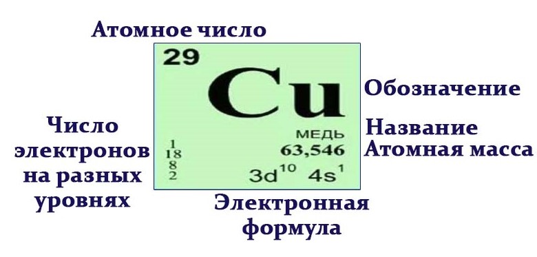

Расшифровка обозначений элементов таблицы Менделеева:

• Обозначение: одной или двумя латинскими буквами.
• Порядковый номер элемента или атомный номер равен числу протонов в его ядре. Обычно пишется в левом верхнем углу. 
• Относительная атомная масса (сумма масс протонов и нейтронов). Это усреднённая величина, для расчёта которой используются атомные массы всех изотопов элемента с учетом их содержания в природе. Поэтому обычно она является дробным числом. 
• Если округлить атомную массу до ближайшего целого, мы получим так называемое массовое число.
• Разность массового числа и атомного числа дает количество нейтронов в ядре. Так, число нейтронов в ядре гелия равно двум, а у лития – четырем. 
• Число положительных протонов, как правило, равно числу отрицательных электронов в атоме (за исключением изотопов). 
• Электронная конфигурация — формула расположения электронов по различным электронным оболочкам атома химического элемента или молекулы.

• Чтобы узнать количество нейтронов в ядре элемента, необходимо из относительной атомной массы (массового числа) вычесть порядковый номер.

Элементы периодической таблицы Менделеева

Металлы расположены в левом нижнем углу таблицы, неметаллы — в правом верхнем углу. Между ними находятся полуметаллы. Все периоды, кроме первого, начинается щелочным металлом. Каждый период заканчивается инертным газом.

• Металлы обладают хорошей электро- и теплопроводностью, способны отражать яркий свет, имеют высокую температуру плавления (остаются твердыми при нормальных значениях окружающей среды, исключение — ртуть).
• Неметаллы встречаются в природе в трех состояниях: газ (например, водород), жидкость (например, бром) и твердые вещества (например, фосфор). Он не способны проводить тепло и электричество. Имеют более низкую температуру плавления в сравнении с металлами, более хрупкие и ломкие. Могут иметь разнообразный внешний вид (элементы с низкой плотностью и яркостью).
• Металлоиды имеют смешанные свойства металлов и неметаллов (например, кремний). Они имеют среднюю  тепло- и электропроводность. Различаются между собой по температуре плавления, плотности, цвету и форме. Внешний вид может быть схож с металлами или неметаллами.

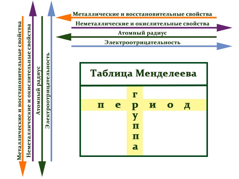
Расшифровка групп и периодов таблицы Менделеева

В таблице химические вещества расположены в специальном порядке: слева направо по мере роста их атомных масс. Все они в периодической системе объединены в периоды и группы.

Периоды — это горизонтальные ряды в таблице. У всех элементов одного периода одинаковое количество заполненных электронами энергетических уровней.
Номер периода, в котором находится элемент, совпадает с номером его валентной оболочки. Эта валентная оболочка постепенно заполняется от начала к концу периода.

Закономерности периодов:

• Металлические свойства убывают, неметаллические и окислительные -возрастают. Каждый период начинается активным металлом и заканчивается инертным газом.
• Уменьшается атомный радиус.
• Увеличивается электроотрицательность.

Группы — это столбцы. Элементы во всех группах имеют одинаковое электронное строение внешних электронных оболочек. В каждой группе на внешнем энергетическом атома одинаковое число электронов, то есть номер группы совпадает с числом валентных электронов, которые могут участвовать в образовании химических связей. Поэтому номер группы часто совпадает с валентностью элементов. Например, номер группы совпадает с валентностью s-элементов и с наибольшей возможной валентностью p-элементов. 

Закономерности групп:

• Металлические свойства увеличиваются, неметаллические и окислительные- убывают.
• Увеличивается радиус атома элементов в рамках одной группы.
• Уменьшается электроотрицательность. 

Атомное число показывает, сколько протонов содержит ядро атома элемента и сколько электронов  в атоме находятся вокруг него. Атом каждого последующего элемента содержит на один протон больше, чем предыдущий.

Валетность  — это свойство элементов образовывать химические связи. То есть это количество химических связей, которые образует атом или число атомов, которое может присоединить или заместить атом данного элемента. Валентность бывает: постоянная и переменная (зависит от состава вещества, в которое входит элемент).
Определить валентность:
— Постоянная валентность идентична номеру группы главной подгруппы. Номера групп в таблице изображаются римскими цифрами.
— Переменная валентность (часто бывает у неметаллов) определяется по формуле: 8 вычесть № группы, в которой находится вещество.

Расшифровка периодов и групп периодической таблицы Менделеева

Каждый элемент имеет свой порядковый (атомный) номер, располагается в определённом периоде и определённой группе.

Периоды

• Малые периоды: первый, второй и третий периоды. В них содержится соответственно 2, 8 и 8 элементов;
• Большие периоды: остальные элементы. В четвёртом и пятом периодах расположены по 18 элементов, в шестом — 32, а в седьмом (пока незавершенном) — 31 элемент. 

В таблице 7 периодов. В каждом содержится определённое число элементов:
1-й период — 2 элемента (малый период),
2-й период — 8 элементов (малый период),
3-й период — 8 элементов (малый период),
4-й период — 18 элементов (большой период),
5-й период — 18 элементов (большой период),
6-й период — 32 элемента (18+14) (большой период),
7-й период — 32 элемента (18+14) (большой период).

Группы и подгруппы

•  Главные подгруппы включают в себя элементы малых периодов и одинаковые с ним по свойствам элементы больших периодов.
• Побочные подгруппы состоят только из элементов больших периодов. Химические свойства элементов главных и побочных подгрупп значительно различаются.

В Периодической таблице может использоваться разное обозначение групп. Поэтому согласно такому обозначению бывает разная расшифровка групп таблицы менделеева:

• 18 групп, пронумерованных арабскими цифрами.
• 8 групп, пронумерованных цифрами с добавлением букв A или B.
  Группы A — это главные подгруппы.
  Группы B — это побочные подгруппы в больших периодов. Это только металлы. 
  IA, VIIIA — по 7 элементов;
  IIA — VIIA — по 6 элементов;
  IIIB — 32 элемента (4+14 лантаноидов +14 актиноидов);
  VIIIB — 12 элементов;
  IB, IIB, IVB — VIIB — по 4 элемента.
  Римский номер группы, как правило, показывает высшую валентность в оксидах (но для некоторых элементов не выполняется). 

Элементы с порядковыми номерами 58–71 (лантаноиды) и 90–103 (актиноиды) вынесены из таблицы и располагаются под ней. Это элементы IIIB группы. Лантаноиды относятся к шестому периоду, а актиноиды — к седьмому.

Элементы главной подгруппы

1 группа главная подгруппа элементов (IA) — щелочные металлы.
Это мягкие металлы, серебристого цвета, хорошо режутся ножом. Все они обладают одним электроном на внешней оболочке и прекрасно вступают в реакцию. 
Литий Li (3), Натрий Na (11), Калий K (19), Рубидий Rb (37), Цезий Cs (55), Франций Fr (87).

2 группа главная подгруппа (IIА) -щелочноземельными металлами.
Имеют серебристый оттенок. На внешнем уровне помещено по два электрона, и, соответственно, эти металлы менее охотно взаимодействуют с другими элементами. По сравнению со щелочными металлами, щелочноземельные металлы плавятся и кипят при более высоких температурах.
 Кальций Ca (20), Стронций Sr (38), Барий Ba (56), Радий Ra (88).

3 группа главная подгруппа (IIIА).
Все элементы данной подгруппы, за исключением бора, металлы. Главную подгруппу составляют составляют бор, алюминий, галлий, индий и таллий. На внешнем электронном уровне элементов по три электрона. Они легко отдают эти электроны или образуют три неспаренных электрона. 

4 группа главная подгруппа (IVА) .
Углерод и кремний обладают всеми свойствами неметаллов, германий и олово занимают промежуточную позицию, а свинец имеет выраженные металлические свойства. Большинство элементов подгруппы углерода — полупроводники (проводят электричество за счёт примесей, но хуже, чем металлы). 

5 группа главная подгруппа (VA).
Физические свойства элементов подгруппы азота различны. Азот является бесцветным газом. Фосфор, мягкое вещество, образует несколько вариантов аллотропных модификаций — белый, красный и чёрный фосфор. Мышьяк — твёрдый полуметалл, способный проводить электрический ток. Висмут — блестящий серебристо-белый металл с радужным отливом. 

6 группа главной подгруппы (VIA) .
Для завершения внешнего электронного уровня атомам этих элементов не хватает лишь двух электронов, поэтому они проявляют сильные окислительные (неметаллические) свойства.

7 группа главная подгруппа (VIIA) — галогены .
(F, Cl, Br, I, At). Имеют семь электронов на внешнем электронном слое атома. Это сильнейшие окислители, легко вступающие в реакции. Галогены («рождающие соли») назвали так потому, что они реагируют со многими металлами с образованием солей. 
Самый активный из галогенов — фтор. Он способен разрушать даже молекулы воды, за что и получил своё грозное имя (слово «фтор» переводится на русский язык как «разрушительный»). А его «близкий родственник» — иод — используется в медицине в виде спиртового раствора для обработки ран.

‍8 группа главная подгруппа (VIIIA)  — инертные (благородные) газы.
(He, Ne, Ar, Kr, Xe, Rn, Og). У них полностью заполнен внешний электронный уровень. Они практически не способны участвовать в реакциях. Поэтому их иногда называют «благородными».  У инертных газов есть способность: они светятся под действием электромагнитного излучения, поэтому используются для создания ламп. Так, неон используется для создания светящихся вывесок и реклам, а ксенон — в автомобильных фарах и фотовспышках. 

Элементы побочной подгруппы

Элементы побочных подгрупп кроме лантаноидов и актиноидов — переходные металлы.
Твёрдые (исключение жидкая ртуть), плотные, обладают характерным блеском, хорошо проводят тепло и электричество. 

Переходные металлы занимают группы 3—12 в периодической таблице. Большинство из них плотные, твердые, с хорошей электро- и теплопроводностью. Их валентные электроны (при помощи которых они соединяются с другими элементами) находятся в нескольких электронных оболочках.

3 группа побочная подгруппа (IIIB) шестого и седьмого периодов — лантаноиды и актиноиды.
Для удобства их помещают под основной таблицей. 

• ‍Лантаноиды иногда называют «редкоземельными элементами», поскольку они были обнаружены в небольшом количестве в составе редких минералов и не образуют собственных руд.
• ‍Актиноиды имеют одно важное общее свойство — радиоактивность. Все они, кроме урана, практически не встречаются в природе и синтезируются искусственно.   

Неметаллы

Правый верхний угол таблицы до инертных газов -неметаллы.
Неметаллы плохо проводят тепло и электричество и могут существовать в трёх агрегатных состояниях: твёрдом (как углерод или кремний), жидком (как бром) и газообразном (как кислород и азот). Водород может проявлять как металлические, так и неметаллические свойства, поэтому его относят как к первой, так и к седьмой группе. 

Кислородные и водородные соединения

Все элементы, кроме гелия, неона и аргона, образуют кислородные соединения.
Существует 8 форм кислородных соединений:  R₂O, RO, R₂O₃, RO₂, R₂O₅, RO₃, R₂O₇, RO₄,
где R — элемент группы.

Элементы главных подгрупп, начиная с IV группы, образуют газообразные водородные соединения. Существуют 4 формы водородных соединений: RH₄, RH₃, RH₂, RH.
Характер соединений: RH — сильнокислый; RH₂ — слабокислый; RH₃ — слабоосновный; RH₄ — нейтральный.